Plotting

Sinaps includes a convenient way to directly plot a neuron geometry and simulation results, through the .plot accesor. This is based on the holoview library.

To illustrate the plotting tool, we first create a simulation of voltage propagation and calcium electrodiffusion, in a simple neuron. Calcium dynamics includes buffering and extrusion.

import sinaps as sn

# Defining the nueron
nrn = sn.Neuron([(0,1),(1,2),(1,3),(3,4)])

# Setting up channels
nrn[0].clear_channels()#Reset all channels, useful if you re-run this cell (does nothing the first time)
nrn[0].add_channel(sn.channels.PulseCurrent(200,2,3),0)
nrn[0].add_channel(sn.channels.PulseCurrent(200,22,23),0)
nrn[0].add_channel(sn.channels.Hodgkin_Huxley())
nrn[0].add_channel(sn.channels.Hodgkin_Huxley_Ca(gCa=14.5,V_Ca=115))

# Defining and running the simulation
sim = sn.Simulation(nrn,dx=10)
sim.run((0,60))

#Setting initial concentrations
for s in nrn.sections:
    s.C0[sn.Species.Ca]=10**(-4)
    s.C0[sn.Species.Buffer]=2*10**(-3)
    s.C0[sn.Species.Buffer_Ca]=0

# Adding chemical reactions: claicum binding to a buffer, and calcium extrusion
nrn.add_reaction(
    {sn.Species.Ca:1,
     sn.Species.Buffer:1},
    {sn.Species.Buffer_Ca:1},
    k1=0.2,
    k2=0.1)

nrn.add_reaction(
    {sn.Species.Ca:1},
    {},
    k1=0.05,k2=0)

# Running electro-diffusion simulations
sim.run_diff(max_step=1)

/home/docs/checkouts/readthedocs.org/user_builds/sinaps/envs/stable/lib/python3.8/site-packages/sinaps/core/model.py:686: UserWarning: The section already had a channel of type <class 'sinaps.core.channels.PulseCurrent'>
  warnings.warn(
100%|██████████| 60.0/60 [00:03<00:00, 19.73ms/s]
  0%|          | 0.3/60 [00:00<02:48,  2.83s/ms]/home/docs/checkouts/readthedocs.org/user_builds/sinaps/envs/stable/lib/python3.8/site-packages/scipy/integrate/_ivp/bdf.py:407: RuntimeWarning: invalid value encountered in subtract
  D[order + 2] = d - D[order + 1]
100%|██████████| 60.0/60 [00:02<00:00, 28.67ms/s]

Neuronal geometry

import hvplot
hvplot.__version__

'0.8.0'

To plot the neuron geometry:

nrn.plot()

Calculating layout...[OK]

Potential

sim.plot.V plots the voltage dynamics at nodes evenly distributed on the neuron. Default number of curves is 10, change number with max_plot.

sim.plot.V(max_plot=2)

Specific sections can be accesed through their names:

sim['Section0000'].plot()

Holoview or matplotlib can be used directly through the pandas Dataframe structure of the data:

sim.V

Section	Section0000										...	Section0003
Position (μm)	5.0	15.0	25.0	35.0	45.0	55.0	65.0	75.0	85.0	95.0	...	5.0	15.0	25.0	35.0	45.0	55.0	65.0	75.0	85.0	95.0
Time
0.000000	0.000000e+00	0.000000e+00	0.000000e+00	0.000000e+00	0.000000e+00	0.000000e+00	0.000000e+00	0.000000e+00	0.000000e+00	0.000000e+00	...	0.000000e+00	0.000000e+00	0.000000e+00	0.000000e+00	0.000000e+00	0.000000e+00	0.000000e+00	0.000000e+00	0.000000e+00	0.000000e+00
0.000009	-2.818983e-07	-2.818983e-07	-2.818983e-07	-2.818983e-07	-2.818983e-07	-2.818983e-07	-2.818983e-07	-2.818983e-07	-2.818958e-07	-2.809372e-07	...	-5.893615e-36	-1.510931e-38	-3.873537e-41	-9.930489e-44	-2.545855e-46	-6.526744e-49	-1.673245e-51	-4.289656e-54	-1.099728e-56	-2.826574e-59
0.000018	-5.637875e-07	-5.637875e-07	-5.637875e-07	-5.637875e-07	-5.637875e-07	-5.637875e-07	-5.637875e-07	-5.637874e-07	-5.637769e-07	-5.607626e-07	...	-8.633726e-35	-2.387195e-37	-6.565528e-40	-1.797409e-42	-4.900798e-45	-1.331476e-47	-3.605930e-50	-9.737830e-53	-2.622955e-55	-7.067587e-58
0.000110	-3.381876e-06	-3.381876e-06	-3.381876e-06	-3.381876e-06	-3.381876e-06	-3.381876e-06	-3.381874e-06	-3.381807e-06	-3.379065e-06	-3.268158e-06	...	-4.509028e-24	-1.105635e-25	-2.711070e-27	-6.647673e-29	-1.630041e-30	-3.996939e-32	-9.800684e-34	-2.403174e-35	-5.892785e-37	-1.480348e-38
0.000202	-6.199049e-06	-6.199049e-06	-6.199049e-06	-6.199049e-06	-6.199049e-06	-6.199049e-06	-6.199039e-06	-6.198706e-06	-6.188122e-06	-5.879501e-06	...	-6.217974e-23	-1.646383e-24	-4.335437e-26	-1.136246e-27	-2.965561e-29	-7.711671e-31	-1.998822e-32	-5.165744e-34	-1.331553e-35	-3.511889e-37
...	...	...	...	...	...	...	...	...	...	...	...	...	...	...	...	...	...	...	...	...	...
54.094150	5.849831e-01	5.849279e-01	5.848146e-01	5.846376e-01	5.843893e-01	5.840596e-01	5.836356e-01	5.831020e-01	5.824406e-01	5.816304e-01	...	5.733876e-01	5.728657e-01	5.723952e-01	5.719783e-01	5.716173e-01	5.713137e-01	5.710690e-01	5.708845e-01	5.707610e-01	5.706991e-01
55.327795	5.518176e-01	5.520532e-01	5.525221e-01	5.532201e-01	5.541414e-01	5.552781e-01	5.566204e-01	5.581565e-01	5.598725e-01	5.617521e-01	...	5.711859e-01	5.716202e-01	5.720011e-01	5.723306e-01	5.726100e-01	5.728409e-01	5.730242e-01	5.731609e-01	5.732517e-01	5.732969e-01
56.970531	4.657728e-01	4.662599e-01	4.672326e-01	4.686886e-01	4.706244e-01	4.730354e-01	4.759159e-01	4.792591e-01	4.830568e-01	4.872991e-01	...	5.126102e-01	5.139124e-01	5.150669e-01	5.160749e-01	5.169372e-01	5.176545e-01	5.182276e-01	5.186570e-01	5.189430e-01	5.190860e-01
58.613268	3.562724e-01	3.568704e-01	3.580656e-01	3.598573e-01	3.622441e-01	3.652243e-01	3.687960e-01	3.729565e-01	3.777027e-01	3.830309e-01	...	4.160449e-01	4.177784e-01	4.193182e-01	4.206646e-01	4.218181e-01	4.227788e-01	4.235471e-01	4.241231e-01	4.245070e-01	4.246990e-01
60.000000	2.616047e-01	2.622108e-01	2.634229e-01	2.652411e-01	2.676655e-01	2.706963e-01	2.743339e-01	2.785785e-01	2.834304e-01	2.888897e-01	...	3.232886e-01	3.251106e-01	3.267302e-01	3.281473e-01	3.293621e-01	3.303743e-01	3.311842e-01	3.317916e-01	3.321965e-01	3.323989e-01

450 rows × 40 columns

sim.V.loc[:,'Section0000'][25].hvplot()

is equivalent to:

sim['Section0000'].V.loc[:,25].hvplot()

The name of the sections can be accessed through the columns function. See the pandas doc for more features.

sim.V.columns

MultiIndex([('Section0000',  5.0),
            ('Section0000', 15.0),
            ('Section0000', 25.0),
            ('Section0000', 35.0),
            ('Section0000', 45.0),
            ('Section0000', 55.0),
            ('Section0000', 65.0),
            ('Section0000', 75.0),
            ('Section0000', 85.0),
            ('Section0000', 95.0),
            ('Section0001',  5.0),
            ('Section0001', 15.0),
            ('Section0001', 25.0),
            ('Section0001', 35.0),
            ('Section0001', 45.0),
            ('Section0001', 55.0),
            ('Section0001', 65.0),
            ('Section0001', 75.0),
            ('Section0001', 85.0),
            ('Section0001', 95.0),
            ('Section0002',  5.0),
            ('Section0002', 15.0),
            ('Section0002', 25.0),
            ('Section0002', 35.0),
            ('Section0002', 45.0),
            ('Section0002', 55.0),
            ('Section0002', 65.0),
            ('Section0002', 75.0),
            ('Section0002', 85.0),
            ('Section0002', 95.0),
            ('Section0003',  5.0),
            ('Section0003', 15.0),
            ('Section0003', 25.0),
            ('Section0003', 35.0),
            ('Section0003', 45.0),
            ('Section0003', 55.0),
            ('Section0003', 65.0),
            ('Section0003', 75.0),
            ('Section0003', 85.0),
            ('Section0003', 95.0)],
           names=['Section', 'Position (μm)'])

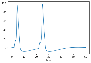
sim.V[('Section0000', 25.0)].plot()

<AxesSubplot:xlabel='Time'>

Field plots are also acccessible through the API. The time can be zoomed through the command time. See the holoview doc for more features.

sim.plot.V_field(time=(0,30))

To help navigating in the field plot, the neuronal geometry is plotted on the left, with a colorbar legend mapping the linear position on the field to the geometry. In a live notebook, the view is interactive. Passing the mouse on the field plot will enhance the corresponding section on the neuronal geometry.

Setting the parameter neuron to False displays only the field plot.

Plotting the currents

The currents computed by the simulation environment are stored in a pandas Dataframe. They are positive when they go toward inside.

sim.plot.I(ChannelClass) plots the currents for the channels of type ChannelClass

sim.plot.I(sn.channels.Hodgkin_Huxley)

The field plots are also accessible:

sim.plot.I_field(sn.channels.Hodgkin_Huxley)

If several channels of the same type are defined on a section, sim.plot.I will plot the sum of all the currents:

sim['Section0000'].plot.I(sn.channels.PulseCurrent)

Holoview or matplotlib can be used directly through the pandas Dataframe structure of the data:

sim.current(sn.channels.Hodgkin_Huxley)

Section	Section0000										...	Section0003
Position (μm)	5.0	15.0	25.0	35.0	45.0	55.0	65.0	75.0	85.0	95.0	...	5.0	15.0	25.0	35.0	45.0	55.0	65.0	75.0	85.0	95.0
Time
0.000000	-0.019335	-0.019335	-0.019335	-0.019335	-0.019335	-0.019335	-0.019335	-0.019335	-0.019335	-0.019335	...	0.0	0.0	0.0	0.0	0.0	0.0	0.0	0.0	0.0	0.0
0.000009	-0.019335	-0.019335	-0.019335	-0.019335	-0.019335	-0.019335	-0.019335	-0.019335	-0.019335	-0.019335	...	0.0	0.0	0.0	0.0	0.0	0.0	0.0	0.0	0.0	0.0
0.000018	-0.019334	-0.019334	-0.019334	-0.019334	-0.019334	-0.019334	-0.019334	-0.019334	-0.019334	-0.019334	...	0.0	0.0	0.0	0.0	0.0	0.0	0.0	0.0	0.0	0.0
0.000110	-0.019328	-0.019328	-0.019328	-0.019328	-0.019328	-0.019328	-0.019328	-0.019328	-0.019328	-0.019328	...	0.0	0.0	0.0	0.0	0.0	0.0	0.0	0.0	0.0	0.0
0.000202	-0.019321	-0.019321	-0.019321	-0.019321	-0.019321	-0.019321	-0.019321	-0.019321	-0.019321	-0.019321	...	0.0	0.0	0.0	0.0	0.0	0.0	0.0	0.0	0.0	0.0
...	...	...	...	...	...	...	...	...	...	...	...	...	...	...	...	...	...	...	...	...	...
54.094150	0.003848	0.004658	0.006118	0.008247	0.011064	0.014587	0.018835	0.023838	0.029638	0.036297	...	0.0	0.0	0.0	0.0	0.0	0.0	0.0	0.0	0.0	0.0
55.327795	-0.074380	-0.073760	-0.072649	-0.071032	-0.068893	-0.066214	-0.062978	-0.059156	-0.054714	-0.049595	...	0.0	0.0	0.0	0.0	0.0	0.0	0.0	0.0	0.0	0.0
56.970531	-0.140742	-0.140372	-0.139731	-0.138805	-0.137581	-0.136045	-0.134181	-0.131967	-0.129370	-0.126348	...	0.0	0.0	0.0	0.0	0.0	0.0	0.0	0.0	0.0	0.0
58.613268	-0.168502	-0.168347	-0.168113	-0.167787	-0.167360	-0.166822	-0.166158	-0.165352	-0.164379	-0.163204	...	0.0	0.0	0.0	0.0	0.0	0.0	0.0	0.0	0.0	0.0
60.000000	-0.168762	-0.168746	-0.168773	-0.168835	-0.168923	-0.169030	-0.169144	-0.169254	-0.169338	-0.169371	...	0.0	0.0	0.0	0.0	0.0	0.0	0.0	0.0	0.0	0.0

450 rows × 40 columns

sim.current(sn.channels.PulseCurrent)['Section0000'].hvplot()

Plotting the species dynamics

The species concentration dynamics computed by the simulation environment are stored in a pandas Dataframe.

sim.plot.C(Species) plots the concentration of Class Species:

sim.plot.C(sn.Species.Ca)

sim['Section0000'].plot.C(sn.Species.Ca)

The species dynamics are stored in a pandas Dataframe, and are accessible via their class:

sim.C[sn.Species.Ca]

Section	Section0000										...	Section0003
Position (μm)	5.0	15.0	25.0	35.0	45.0	55.0	65.0	75.0	85.0	95.0	...	5.0	15.0	25.0	35.0	45.0	55.0	65.0	75.0	85.0	95.0
Time
0.000000	0.000100	0.000100	0.000100	0.000100	0.000100	0.000100	0.000100	0.000100	0.000100	0.000100	...	0.000100	0.000100	0.000100	0.000100	0.000100	0.000100	0.000100	0.000100	0.000100	0.000100
0.019853	0.000100	0.000100	0.000100	0.000100	0.000100	0.000100	0.000100	0.000100	0.000100	0.000100	...	0.000100	0.000100	0.000100	0.000100	0.000100	0.000100	0.000100	0.000100	0.000100	0.000100
0.039706	0.000100	0.000100	0.000100	0.000100	0.000100	0.000100	0.000100	0.000100	0.000100	0.000100	...	0.000100	0.000100	0.000100	0.000100	0.000100	0.000100	0.000100	0.000100	0.000100	0.000100
0.238233	0.000099	0.000099	0.000099	0.000099	0.000099	0.000099	0.000099	0.000099	0.000099	0.000099	...	0.000099	0.000099	0.000099	0.000099	0.000099	0.000099	0.000099	0.000099	0.000099	0.000099
0.436761	0.000098	0.000098	0.000098	0.000098	0.000098	0.000098	0.000098	0.000098	0.000098	0.000098	...	0.000098	0.000098	0.000098	0.000098	0.000098	0.000098	0.000098	0.000098	0.000098	0.000098
...	...	...	...	...	...	...	...	...	...	...	...	...	...	...	...	...	...	...	...	...	...
56.436761	0.000006	0.000006	0.000006	0.000006	0.000006	0.000006	0.000006	0.000006	0.000006	0.000006	...	0.000006	0.000006	0.000006	0.000006	0.000006	0.000006	0.000006	0.000006	0.000006	0.000006
57.436761	0.000006	0.000006	0.000006	0.000006	0.000006	0.000006	0.000006	0.000006	0.000006	0.000006	...	0.000006	0.000006	0.000006	0.000006	0.000006	0.000006	0.000006	0.000006	0.000006	0.000006
58.436761	0.000005	0.000005	0.000005	0.000005	0.000005	0.000005	0.000005	0.000005	0.000005	0.000005	...	0.000005	0.000005	0.000005	0.000005	0.000005	0.000005	0.000005	0.000005	0.000005	0.000005
59.436761	0.000005	0.000005	0.000005	0.000005	0.000005	0.000005	0.000005	0.000005	0.000005	0.000005	...	0.000005	0.000005	0.000005	0.000005	0.000005	0.000005	0.000005	0.000005	0.000005	0.000005
60.000000	0.000005	0.000005	0.000005	0.000005	0.000005	0.000005	0.000005	0.000005	0.000005	0.000005	...	0.000005	0.000005	0.000005	0.000005	0.000005	0.000005	0.000005	0.000005	0.000005	0.000005

65 rows × 40 columns

sim.C[sn.Species.Ca].loc[:,'Section0000'][25].hvplot()

is equivalent to:

sim['Section0000'].C(sn.Species.Ca).loc[:,25].hvplot()

sim['Section0000'].C(sn.Species.Buffer_Ca).loc[:,5].hvplot()