Model Description

To model voltage propagation and ionic electrodiffusion in the Sinaps python package, we consider the Cable equation [1] for voltage dynamic, coupled to the Nernst-Planck equation for ionic dynamic.
The Cable equation makes an analogy between the dendritic tree, and a electric wire composed of RC circuits:

$$c \frac{\partial V}{\partial t} = I^G + \frac{1}{R} \frac{\partial^2 V}{\partial x^2}.$$

In this model, the axonal membrane acts as a capacitor (capacitance $c$), in parallel with voltage-dependent conductors accounting for ionic channels (currents $I^G$). The voltage propagation is represented by a resistive current: the current transported by electrons in the solid structure of the wire follows Ohm’s law (current $I = \frac{U}{R}$). This model assumes a zero extracellular potential. There are a priori no restrictions on membrane currents.
To infer calcium dynamics from voltage propagation, we couple the previous equation to the Nernst-Planck equation, for ionic electrodiffusion. This equation describes the motion of charged species within an electrolyte [2], and is build from the first principle of mechanics, stating the conservation of ions. We add to this equation the flux of ions coming from the channels, as well as the variation of concentration due to the eventual chemical reactions. We get:

$$\label{NP} \frac{\partial c^i}{\partial t} = - \nabla \cdot j^i + j^{i,\text{m}} + \gamma^{i,\text{chem}} ;; \forall i \in \text{{ions}}$$

The flux of charge per surface area $j_i$ [mol.s$^{-1}$.m$^{-2}$], sums the diffusion flux of ionic species derived from Fick’s law $j_{diff}^i = - D_i \nabla c_i$, and an electric flux representing the motion of ions due to the electric field: $j_{\text{elec}}^i = - \frac{D_i z_i e c_i}{k_b T} \nabla V$ [2,3]. $\displaystyle \frac{D_i z_i e c_i}{k_b T}$ is the Einstein relation for the mobility of ion species: $D_i$ is the diffusion coefficient of species $i$, $z_i$ the valence of species $i$, $k_B T$ the thermal energy and $e$ is the electric charge [3]. We get:

$$j^i = j_{diff}^i + j_{\text{elec}}^i = - D_i \nabla c^i - \frac{D^i z^i e c^i}{k_b T} \nabla V.$$

$j^{i, \text{m}}$ represents the lineic flux of ions entering from the channels [mol.s$^{-1}$.m$^{-1}$]. $\gamma^{i,\text{chem}}$ represents the variations of concentration due to the eventual chemical reactions.

Notations

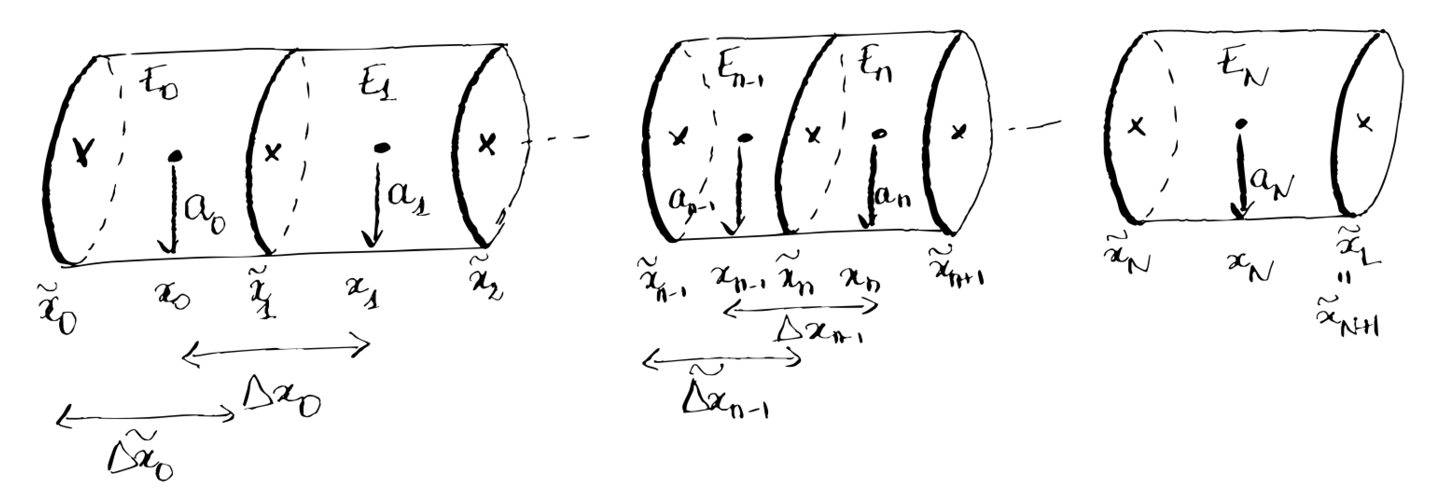
In one branch going between $\tilde{x}_0 \leq x \leq \tilde{x}_L$, we consider different positions $\tilde{x}_0 < \tilde{x}_1<…< \tilde{x}_n <…< \tilde{x}N < \tilde{x}{N+1} = \tilde{x}L$. We then define $x_n$ as the middle point between $\tilde{x}n$ and $\tilde{x}{n+1}$ (see Fig. [1]). Finally, we define the elementary domains $E_n$, $n = 0..N$, with boundaries $\tilde{x}n$ and $\tilde{x}{n+1}$. The domains $E_n$ are portions of cylinders, with radius $a_n$, centered around $x_n$, with length $\tilde{\Delta x_n} = \tilde{x}{n+1} - \tilde{x}n.$ We also define $\Delta x_n = x{n+1} - x_n.$

Our goal is to compute the potential $V_n$ and the concentration of each ionic species $i$, $c_n^i$, at each point $x_n$.

Fig. 1: Discretization of one branch. The potential and the concentrations are evaluated at each point $x_n$ in the branch.

Derivation of the discretized Cable equation in branches

We derive the discretized Cable equation for voltage dynamics along one branch. We evaluate the potentials $V_n$, $n = 0..N$ at each point $x_n$. The propagation of voltage in each elementary domain $E_n$ is modeled using an analogy with a RC electrical circuit:

Fig. 2: Analogy with a RC electrical circuit. Each elementary domain of size $\tilde{\Delta x}$ contains a capacitor and a conductor to account for the capacitive and conductive properties of the membrane.

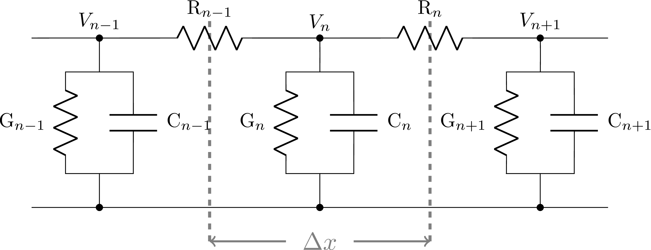
The axonal membrane behaves as a capacitor, and generates a current

$$\displaystyle I_n^C =C_n \frac{d V_n}{dt},;;; 0 \leq n \leq N,$$

where $C_n$ represents the capacity of the membrane in domain $E_n$. This capacitor is in parallel with voltage-dependent conductors to account for the active channels present on the membrane, that will be denoted by

$$\displaystyle I_n^G(t) = 2 \pi a_n \tilde{\Delta x_n} I^G(t, V_n);;; 0 \leq n \leq N$$

where $I^G(t, V_n)$ is the membrane current in $E_n$ (in $A.m^{-2}$).
Finally, the voltage propagation from $E_{n-1}$ to $E_{n}$ and from $E_{n+1}$ to $E_{n}$ are represented by the resistive currents $I_{n-1}^R$ and $I_{n}^R$ such that

$$\displaystyle I_{n}^R = \frac{1}{R_{n}}\left(V_{n} - V_{n-1} \right);;; 1 \leq n \leq N-1,$$

where $R_{n}$ is the cytoplasmic resistance in domain $E_{n}$.
The electrical components $R_n$ and $C_n$ are derived using standard computation of the resulting capacitance and conductance in a cylinder. The membrane capacitance $C_n$ (in $\text{Farad}$) is given by:

$$\begin{aligned} C_n = c_n 2 \pi a_n \tilde{\Delta x_n}\end{aligned}$$

where $c_n$ is the permittivity of the membrane in domain $E_n$ (in $\text{F}.\text{cm}^{-2}$).
The cytoplasm axial resistance $R_{n-1,n}$ (in $\Omega$) from domain $E_{n-1}$ to $E_n$ is:

$$\begin{aligned} R_{n} = r_{n} \frac{\Delta x_{n}}{\pi a_{n}^2}\end{aligned}$$

where $r_{n}$ is the cytoplasmic electrical conductance ($[\Omega . \text{cm}]$) in domain $E_{n}$.
Using Kirchhoff’s current law in position $x_n$, we get:

$$I_n^C - I_n^G - I_{n-1}^R + I_{n}^R =0.$$

Replacing the currents with their formulas in the previous equation, we get the discretized Cable equation for the dynamics and propagation of voltage in domain $E_n$:

$$\begin{aligned} \label{eqCable} C_n \frac{d V_n(t)}{dt} = I_n^G(t) + \frac{V_{n} - V_{n-1}}{R_{n-1}} - \frac{V_{n+1} - V_n}{R_{n}}.\end{aligned}$$

At the tip of the branch, the currents $I_0 = 0$ and $I_N = 0$. Hence, Kirchoff’s law rewrites:

$$I_k^C - I_k^G - I_{k}^R =0;;; \text{for } k = 1,N.$$

The equation becomes:

$$\begin{aligned} &C_1 \frac{d V_1(t)}{dt} = I_1^G(t) - \frac{V_{2} - V_{1}}{R_{1}}\ &C_{N} \frac{d V_{N}(t)}{dt} = I_{N}^G(t) + \frac{V_{N} - V_{N-1}}{R_{N-1}}\end{aligned}$$

If the radius $a_n$, the length $\Delta x_n$, the cytoplasmic electric conductivity $r_n$ and the membrane permittivity $c_n$ are independent of $n$ along the branch, i.e. $a_n = a$, $\Delta x_n=\Delta x$, $r_n = r$ and $r_n = r$ for all $n$ in the branch, we recognize the discretized form of the Cable equation:

$$\begin{aligned} \label{MSeq_tip} c \frac{\partial V}{\partial t} = I^G + \frac{a}{2 r} \frac{\partial^2 V}{\partial x^2},\end{aligned}$$

with reflective boundary condtions at the tips $x = 0$ and $x = L$:

$$\begin{aligned} \frac{\partial V}{\partial x}(t,0) = 0\ \frac{\partial V}{\partial x}(t,L) = 0\end{aligned}$$

Derivation of the discretized Cable equation at junctions

Fig. 3: Strategy at branches junction. We introduce a virtual point $x_p$, in the middle of the junction, where we evaluate the potential $V_p$.

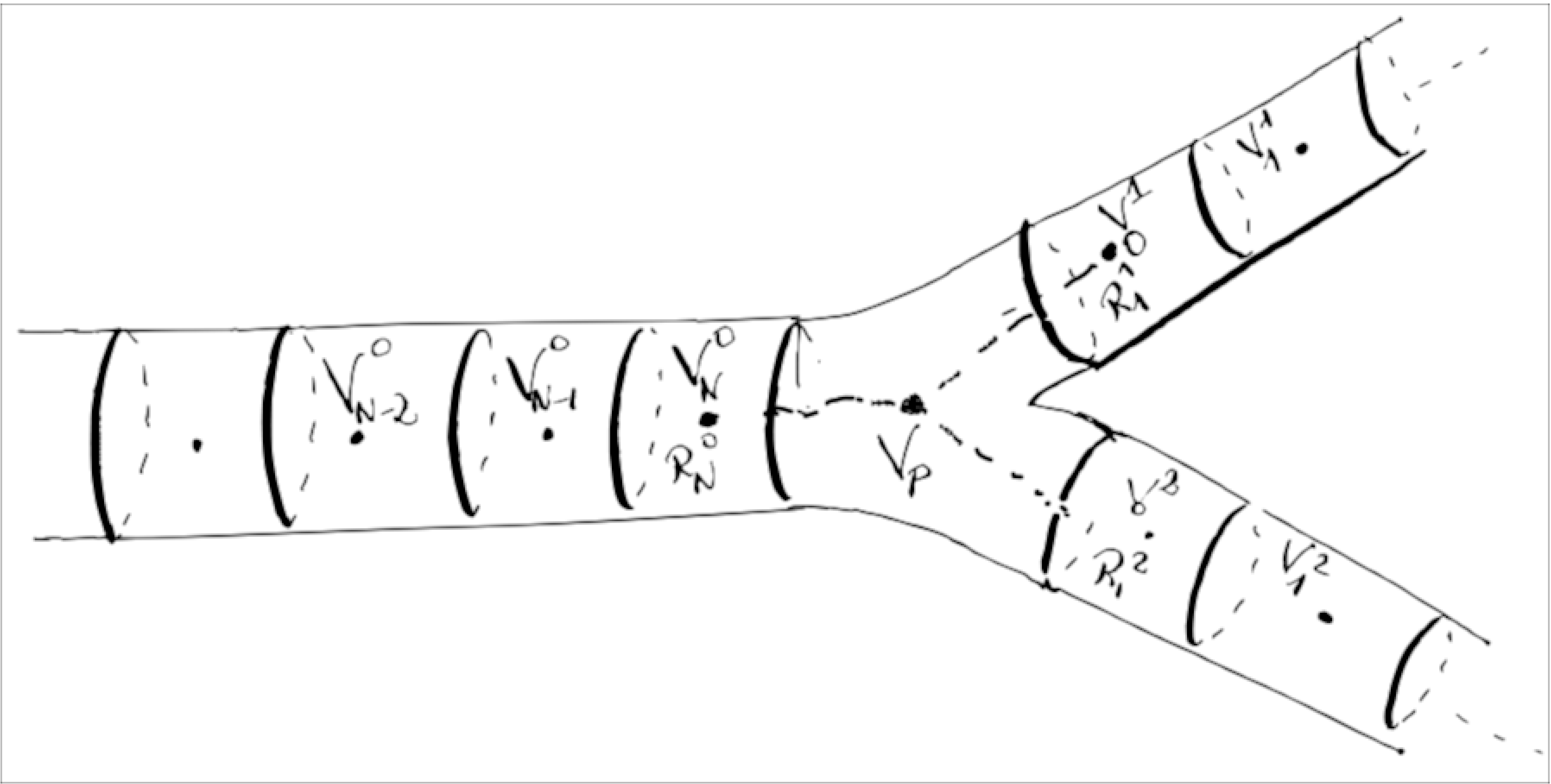
To derive the discretized equation at the junction between three branches, we introduce a virtual point $x_p$ in the middle of the junction. We consider that the junction is located at the end of branch $0$, and at the start of branch $1$ and $2$ (see Fig. [3]). We define the resistive current between the point $x_N^0$, the last point in branch $0$, and $x_p$. The same way between $x_1^1$ and $x_1^2$, the first points of branches $1$ and $2$ respectively and $x_p$. We obtain:

$$\begin{aligned} I_N^{0,R} &= \frac{V_p - V_N^0}{R_N^0}\ I_1^{1,R} &= \frac{V_1^1 - V_p}{R_1^1}\ I_1^{2,R} &= \frac{V_1^2 - V_p}{R_1^2}\end{aligned}$$

Using Kirchhoff’s law at point $x_p$, we get $I_N^{0,R} - I_1^{1,R} - I_1^{2,R} = 0$, and hence

$$V_p = \frac{V_N^0/R_N^0 + V_1^1/R_1^1 + V_1^2/R_1^2}{1/R_N^0 + 1/R_1^1 + 1/R_1^2}$$

Finally, we get the equations for $V_N^0$, $V_1^1$ and $V_1^2$ using Kirchoff’s law at points $x_N^0$, $x_1^1$ and $x_1^2$. Follows the example for $V_N^0$:

$$C_N^0 \frac{d V_N^0(t)}{dt} = I_N^{G,0}(t) + \frac{V_{N}^0 - V_{N-1}^0}{R_{N-1}} - \frac{V_p - V_N^0}{R_N^0}.$$

This set of coupled linear equations for the voltage is then solved using the BDF solver.

Derivation of the discretized Nernst-Planck equation

Using the same formalism as before, we discretize the Nernst-Planck equation. To simplify the notations, we will consider in this section that the radius is constant, even though the code supports variations in the radius along the branches. In each elementary domain, for each ionic species $i$, we solve the equation for the concentration dynamic $c_n^i$ with the discretized flux:

$$\begin{aligned} \frac{\partial c_n^i}{\partial t} = - \frac{j^i_{n+1} - j_n^i}{\tilde{\Delta x_n}} + \frac{2 j_n^{i, \text{m}}}{a_n} + \gamma_n^{i, \text{chem}}\end{aligned}$$

where:

$$ j_n^i = - D_n^i \frac{c_n^{i} - c_{n-1}^i}{\tilde{\Delta x_n}} - \frac{D_n^i z^i e}{k_B T} c_n^i \frac{V_{n} - V_{n-1}}{\tilde{\Delta x_n}}. $$

$j_n^{i,m}$ is the flow of ions of species $i$ coming from channels (in [mol . s$^{-1}$]), that is define within the channel class.
The chemical flux $\gamma_n^{i, \text{chem}}$ will be described in the next section.

Implementation of chemical reactions

The model equation for chemical reactions is the classical chemical equations. Considering the reaction

$$ \require{mhchem} \begin{aligned} \sum_{i = 1}^n \alpha_i \text{A}i \xrightleftharpoons[\mathbf{k{b}}]{\mathbf{k_{f}}} \sum_{i = 1}^m \beta_i \text{B}_i, \label{eqChem}\end{aligned}$$

between ionic species $A_i$, $i = 1,…,n$ and $B_i$, $i = 1,..,m$, we compute in each elementary domain $E_n$ the reaction speeds:

$$\begin{aligned} v^f_n &= \displaystyle k_f \prod_{i = 1}^n \left(c_n^{A_i}\right)^{\alpha_i}\ v^b_n &= \displaystyle k_b \prod_{i = 1}^m \left(c_n^{B_i}\right)^{\beta_i}.\end{aligned}$$

The variation of concentration of each species, due to the chemical reaction inside $E_n$ is then:

$$\gamma_n^{A_i,\text{chem}} = \alpha_i (v_n^b - v_n^f)$$

for the reactants $A_i$, and

$$\gamma_n^{B_i,\text{chem}} = \beta_i (v_n^f - v_n^b)$$

for the products $B_i$.

Bibliography

[1] Tuckwell HC, Introduction to Theoretical Neurobiology, Cambridge University Press, 1988

[2] Nernst W, Zur Kinetik der in Lösung befindlichen Körper, Zeitschr f Phys Chem 2, pp. 613-637, 1888

[3] Kirby BJ, Micro- and Nanoscale Fluid Mechanics, Cambridge University Press, 2010